Dear all,
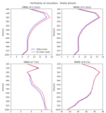
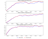
I've made 1-month period of simulation with MPAS-A, using both 30km quasi-uniform and 60-10km variable-resolution meshes. However, due to limited articles/materials denoting error characteristics of MPAS-A, I don't have much understanding of my results. I compared some model outputs against ERA5 analysis by interpolating MPAS-A results to the same 0.25deg grid and calculate RMSEs within 80°S~80°N. The figures that attached show a timeseries and a time-averaged vertical profile, respectively. For the timeseries plot, I've considered 500hPa zonal wind and temperature, and 850hPa humidity. While the other plot includes the profile of wind, temperature and relative humidity.
The simulation starts at 2016-6-19 00UTC and finalize at 2016-7-22 00UTC. It is clear from the timeseries plot that simulation errors arise continuously for nearly two weeks before reaching a relative stable state. And it is shown in the other plot that vertical distribution of simulation errors is quite different for the variables taken into account.
For my own point of view, the RMSEs derived from my experiments may be a bit large (Compared to the results in Ha et al. 2017 article). I have no idea whether the results shown are reasonable, if really not, what could be the reason leading to a larger error? Can I reduce the error by optimizing the model namelist configurations? Any comments is greatly appreciated.
------
Here's my non-default namelist settings:
- initial conditions from FNL analysis.
- dt=150s, dx=30000 for 30km mesh; dt=60s, dx=10000 for 60-10km mesh.
- "mesoscale reference" physics suite, but changing convection scheme to Grell Freitas.
- config_radtlw_interval and config_radtsw_interval set to '00:30:00'.
- SST is updated everyday by 00UTC, extracted from FNL datasets.