How to extract wind(zonal & meridional), geopotential height using the convert_mpas include_field

[makinde]

Good day,
Thanks for being a help to us newbies.
I am writing to find how to post-process wind components and geopotential Height across all levels from the MPAS model.

I have ran a 10 day variable resolution simulation with MPAS and I am about to analyze, since I don't know much about how the model runs or the variables the model produces, I have gotten some stream_list.atmosphere.(diagnostics, output) ( all attached including the namelist and the streams.atmosphere) to run the model. In those files, I found numerous variable name there, but couldn't found (or notice) any one of them to give the idea of u(zonal wind component) or v(meridional wind component), geopotential height and vertical windspeed at levels.

I have configured the simulations to output diagnostics file at every day as below:

//////////////////////////////////
diag.2009-01-01_00.00.00.nc
diag.2009-01-02_00.00.00.nc
diag.2009-01-03_00.00.00.nc
diag.2009-01-04_00.00.00.nc
///////////////////////////////////


I want to post-process u, v, geopotential height and the vertical from the diag file using convert_mpas tool to get a single file (latlon.nc), but I don't know which of the variable names in the output and the diagnostic stream_list I should include in the convert_mpas include_field.

Please can anyone put me through this?

I have gone through the user guide, but couldn't find useful information about these particular variables, may they need to be calculated?
If so, at least I will need some other parameters (variables) like wind speed to calculate some of the above listed variables.

please any help will be appreciated.


Thanks so much for your usual help.

 

[mgduda]

I sincerely apologize for the long delay in replying!

The zonal and meridional components of the horizontal wind field are available as the 'uReconstructZonal' and 'uReconstructMeridional' fields. These are not included in the diagnostics output files by default, but you can add them to your stream_list.atmosphere.diagnostics file before starting the model simulation. Internally, the model interpolates the prognosed normal component of horizontal wind at cell faces ("edges") to cell centers using radial basis functions; so, the 'uReconstructZonal' and 'uReconstructMeridional' fields are horizontally located at the nominal centers of grid cells. In the vertical, these fields are located at the midpoint of layers in the model's smoothed terrain-following vertical coordinate.

At present, there is no geopotential height field available directly from the model. However, in the model initial conditions file ('x6.999426.init.nc'), there should be a field named 'zgrid'. The 'zgrid' field provides the geometric height at the layer interfaces in each column of the model grid, which you could use to compute geopotential height. The geometric height of layer midpoints (where the 'uReconstructZonal' and 'uReconstructMeridional' fields are located vertically) is simply the average of the heights of layer interfaces at the bottom and at the top of each layer.

Apologies, again, for the slow reply, and please don't hesitate to follow-up in this thread if there are any details that I can clarify!

 

[makinde]

Thank you Mgduda for the reply.

Please am just coming back to this for a long time due to instability.
Am trying to follow up on the thread, thanks for the response, I understand from your last reply that I have to manually include the 'uReconstructZonal' and the 'uReconstructMeridional' into the stream_list.atmosphere.diagnostic file, which will cater for the horizontal zonal and meridional wind component, If you still remember very well my question, it include how to get this zonal and meridional wind at all levels.

I have defined pressure levels as follows
[1000, 975, 950, 925, 900, 850, 800, 750, 700, 650, 600, 550, 500, 450, 400, 350, 300, 250, 200, 150, 100, 70, 50, 30, 20, 10]
I need both zonal and meridional winds at all this levels.

I got your explanation about the horizontal wind components and how the vertical position of it from your words in quote "In the vertical, these fields are located at the midpoint of layers in the model's smoothed terrain-following vertical coordinate."
So please how do I include these vertically positioned 'uReconstructZonal' and 'uReconstructMeridional' in the diagnostic file and also in the include_list file for the convert_mpas?

Another question is that, please can you confirm that 'w_200hpa' for example is the vertical velocity(omega) at 200hpa?

Thank you so much.
Please am very sorry for just following up, please bear with me.
Thank you.

 

[mgduda]

I'm very sorry again for the delay in my reply. I've attached a Python script that may be helpful in vertically interpolating the zonal and meridional winds from the native model levels in the diagnostics files to isobaric levels.

A complete workflow might involve the following steps:

1. Ensure that the uReconstructZonal and uReconstructMeridional fields, as well as the 3-d pressure field, are saved to diagnostics files. You could either add these fields to the "stream_list.atmosphere.diagnostics" file, or you could list these three fields directly in the "streams.atmosphere" file, e.g.,
   

   <stream name="diagnostics"
           type="output"
           filename_template="diag.$Y-$M-$D_$h.$m.$s.nc"
           output_interval="3:00:00" >
   
           <file name="stream_list.atmosphere.diagnostics"/>
           <var name="uReconstructZonal"/>
           <var name="uReconstructMeridional"/>
           <var name="pressure"/>
   </stream>

2. After completing the model simulation, interpolate the winds to isobaric levels with the attached "isobaric_interp.py" script, e.g.,
   

   isobaric_interp.py diag.2009-01-01_00.00.00.nc iso_winds.2009-01-01_00.nc
   isobaric_interp.py diag.2009-01-02_00.00.00.nc iso_winds.2009-01-02_00.nc
   isobaric_interp.py diag.2009-01-03_00.00.00.nc iso_winds.2009-01-03_00.nc

   The Python script can only operate on a single input file at a time (the second command-line argument is an optional output file name). However, with a simple shell script, you can parallelize the interpolation across files.
   
3. Optionally, concatenate all time periods of the vertically interpolated wind field into a single netCDF file with "ncrcat", e.g.,
   

   ncrcat iso_winds.2009*nc iso_winds.nc

4. Horizontally interpolate the vertically interpolated wind fields to a latitude-longitude grid using the convert_mpas program, e.g.,
   

   convert_mpas init.nc iso_winds.nc

   The horizontal interpolation will not work, however, near grid cells where the isobaric surfaces are below the lowest model level or above the highest model level. If you have a preferred method for vertical extrapolation, you could modify the "isobaric_interp.py" script to provide extrapolated values below ground or above the model top to avoid this issue. Alternatively (and probably involving substantially more work), the "convert_mpas" program could be modified to avoid the use of fill values in its horizontal interpolation.

Hopefully this will provide some guidance on how to proceed. There is still the issue of how to get geopotential height at isobaric levels. Roughly, I think a reasonable approach might be to compute geopotential height from the "zgrid" field in the model initial conditions file. Conveniently, the "zgrid" field gives the geometric height at layer interfaces, which simplifies the computation of geopotential height with a vertical integral. Once you have computed geopotential height at layer mid-points, the same vertical interpolation that is used for the wind fields can be applied using the time-varying 3-d pressure field.

 

[makinde]

Thank you Mgduda for the detailed response.
Please am very sorry for the so much delayed reply. I am just reading your response now, it was so because I kept on checking for a reply but when it did not come in time I forgot about it. Unfortunately, I have not been able to solve the problem up till now. So searching through this forum again, I came across your reply.

Thank you so much, I will try all the steps you have detailed in the response.
Thank you once again, am very grateful.

 

[makinde]

I'm very sorry again for the delay in my reply. I've attached a Python script that may be helpful in vertically interpolating the zonal and meridional winds from the native model levels in the diagnostics files to isobaric levels.

A complete workflow might involve the following steps:

1. Ensure that the uReconstructZonal and uReconstructMeridional fields, as well as the 3-d pressure field, are saved to diagnostics files. You could either add these fields to the "stream_list.atmosphere.diagnostics" file, or you could list these three fields directly in the "streams.atmosphere" file, e.g.,
   

   <stream name="diagnostics"
           type="output"
           filename_template="diag.$Y-$M-$D_$h.$m.$s.nc"
           output_interval="3:00:00" >
   
           <file name="stream_list.atmosphere.diagnostics"/>
           <var name="uReconstructZonal"/>
           <var name="uReconstructMeridional"/>
           <var name="pressure"/>
   </stream>

2. After completing the model simulation, interpolate the winds to isobaric levels with the attached "isobaric_interp.py" script, e.g.,
   

   isobaric_interp.py diag.2009-01-01_00.00.00.nc iso_winds.2009-01-01_00.nc
   isobaric_interp.py diag.2009-01-02_00.00.00.nc iso_winds.2009-01-02_00.nc
   isobaric_interp.py diag.2009-01-03_00.00.00.nc iso_winds.2009-01-03_00.nc

   The Python script can only operate on a single input file at a time (the second command-line argument is an optional output file name). However, with a simple shell script, you can parallelize the interpolation across files.
   
3. Optionally, concatenate all time periods of the vertically interpolated wind field into a single netCDF file with "ncrcat", e.g.,
   

   ncrcat iso_winds.2009*nc iso_winds.nc

4. Horizontally interpolate the vertically interpolated wind fields to a latitude-longitude grid using the convert_mpas program, e.g.,
   

   convert_mpas init.nc iso_winds.nc

   The horizontal interpolation will not work, however, near grid cells where the isobaric surfaces are below the lowest model level or above the highest model level. If you have a preferred method for vertical extrapolation, you could modify the "isobaric_interp.py" script to provide extrapolated values below ground or above the model top to avoid this issue. Alternatively (and probably involving substantially more work), the "convert_mpas" program could be modified to avoid the use of fill values in its horizontal interpolation.

Hopefully this will provide some guidance on how to proceed. There is still the issue of how to get geopotential height at isobaric levels. Roughly, I think a reasonable approach might be to compute geopotential height from the "zgrid" field in the model initial conditions file. Conveniently, the "zgrid" field gives the geometric height at layer interfaces, which simplifies the computation of geopotential height with a vertical integral. Once you have computed geopotential height at layer mid-points, the same vertical interpolation that is used for the wind fields can be applied using the time-varying 3-d pressure field.

Thank you so much for being there. I have been facing some technical issues running MPAS for a while which have to do with my account but it has been solved.
Thank you for the isobaric interpolation script. I have been able to modify it and write a shell script to parallelize it. It is working fine.

Please can you guide me more on how to get geopotential height and vertical wind from MPAS output?

Thank you.

 

[mgduda]

I'm very sorry for not responding for so long, but hopefully the following will still be helpful.

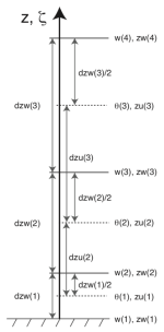
Regarding vertical velocity, the model produces a field named 'w' that contains the vertical velocity in m/s at model layer interfaces. I've reproduced here Figure C.5 from the user's guide:



The 'w' field is defined at the levels labeled w(1), w(2), etc. in the figure. Most other variables (temperature, horizontal winds, humidity, etc.) are defined at the levels labeled theta(1), theta(2), etc. in the figure. The "theta" levels are defined at the geometric midpoint of layers, so, for example, you could compute the average of w(1) and w(2) to get a vertical velocity valid at the theta(1) level in a column of the model output.

Regarding geopotential height, there is a code branch under development that provides a routine for computing geopotential height from geometric height:

   !***********************************************************************
   !
   !  routine compute_geopotential_height
   !
   !> \brief   Convert geometric height to geopotential height
   !>          Adopted from convert_gpsro_bufr.f90 in DART/observations/gps/. 
   !> \author  Soyoung Ha
   !> \date    17 Feb 2017
   !
   !> \details
   !>  Given latitude (in degree), convert geometric height (in meter)
   !>  into geopotential height (in meter).
   !>  
   !>  Input:   
   !>  ncol -- nCells
   !>  nlev -- nIsobaricLevels
   !>  lat  -- latitude [radian]   
   !>  H    -- geometric height [m]
   !>  
   !>  Output:   
   !>  GPH  -- geopotential height [m]
   !>  
   !----------------------------------------------------------------------- 
    subroutine compute_geopotential_height(ncol, nlev, lat, H, GPH)

       implicit none

    !  Input and Output arguments:
       integer,          intent(in):: ncol, nlev
       real(kind=RKIND), intent(in),  dimension(ncol)       :: lat
       real(kind=RKIND), intent(in),  dimension(nlev,ncol)  :: H
       real(kind=RKIND), intent(out), dimension(nlev,ncol)  :: GPH

    !  Local variables
       integer :: k, iCell
       real(kind=RKIND), dimension(ncol) :: sin2, termr, termg
       real(kind=RKIND) :: semi_major_axis, semi_minor_axis, grav_polar, grav_equator
       real(kind=RKIND) :: earth_omega, grav_constant, flattening, somigliana
       real(kind=RKIND) :: grav_ratio, grav, eccentricity

    !  Parameters below from WGS-84 model software inside GPS receivers.
       parameter(semi_major_axis = 6378.1370e3_RKIND)    ! (m)
       parameter(semi_minor_axis = 6356.7523142e3_RKIND) ! (m)
       parameter(grav_polar = 9.8321849378_RKIND)        ! (m/s2)
       parameter(grav_equator = 9.7803253359_RKIND)      ! (m/s2)

       parameter(earth_omega = 7.292115e-5_RKIND)        ! (rad/s)  
       parameter(grav = 9.80665_RKIND)                 ! (m/s2) WMO std g at 45 deg lat

       parameter(grav_constant = 3.986004418e14_RKIND)   ! (m3/s2)
       parameter(eccentricity = 0.081819_RKIND)        ! unitless

    !  Derived geophysical constants
       parameter(flattening = (semi_major_axis-semi_minor_axis) / semi_major_axis)

       parameter(somigliana = (semi_minor_axis/semi_major_axis)*(grav_polar/grav_equator)-1.0_RKIND)

       parameter(grav_ratio = (earth_omega*earth_omega * &
                               semi_major_axis*semi_major_axis * semi_minor_axis)/grav_constant)

       sin2(:)  = sin(lat(:))**2
       termg(:) = grav_equator * ( (1.0_RKIND+somigliana*sin2(:)) / &
                      sqrt(1.0_RKIND - eccentricity**2 * sin2(:)) )
       termr(:) = semi_major_axis / (1.0_RKIND + flattening + grav_ratio - 2.0_RKIND*flattening*sin2(:))

       do iCell = 1, ncol
          do k = 1, nlev
             GPH(k,iCell) = (termg(iCell)/grav)*((termr(iCell)*H(k,iCell))/(termr(iCell)+H(k,iCell)))
          end do
       end do

    end subroutine compute_geopotential_height

It should be possible to include the "compute_geopotential_height" routine directly in the MPAS source code, or to adapt it to, e.g., a Python routine.

If there are any points on which I could offer any clarification, please don't hesitate to let me know, and I'll be glad to help!

 

[makinde]

Dear Mgduda,

Thank you so much for those great replies, you are too much.
Do you know I have not been able to compute the geopotential height up till now? 3 months have passed, I am still looking and searching online for how to go about it. Though at a time, I have to shelf it and finish a paper. However, I have come to this forum several times but there was no response to my post yet, I could not find your response at all. I was just scrolling through the posts again today, only to discovered you have responded a long time ago.
Thank you so much for the great response.

As you mentioned in your response, can you please guide me on how to include the "compute_geopotential_height" routine directly into the MPAS source code?
Secondly, in the routine you posted, it was commented in the description that lat should be in degrees but somewhere under the Input comment, it was written to radians. Please which one of these units (degrees or radians) is the correct unit for the lat?

Thanks.