********************************************************************************************************************************************************************
Dear Colleagues,
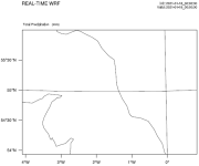
For plotting wrfout file, I am not sure whether NCL draws the initial time (see my code below), because I really found that the figure at the initial time "2019-06-11_00:00:00" has no color legend bar. Could you please kindly confirm this issue? Many thanks. I also attach the figures at initial time and the next hour for your check.
Best regards,
Stella
********************************************************************************************************************************************************************
; Example script to produce plots for a WRF real-data run,
; with the ARW coordinate dynamics option.
; In this example we first get the entire field over time, which will
; make it easier to calculate tendencies
load "$NCARG_ROOT/lib/ncarg/nclscripts/csm/gsn_code.ncl"
load "$NCARG_ROOT/lib/ncarg/nclscripts/wrf/WRFUserARW.ncl"
begin
;
; The WRF ARW input file.
; This needs to have a ".nc" appended, so just do it.
a = addfile("./wrfout_d03_2019-06-11_00:00:00.nc","r")
; We generate plots, but what kind do we prefer?
; type = "x11"
type = "pdf"
; type = "ps"
; type = "ncgm"
wks = gsn_open_wks(type,"plt_Precip3")
; Set some basic resources
res = True
res@MainTitle = "REAL-TIME WRF"
pltres = True
mpres = True
mpres@mpGeophysicalLineColor = "Black"
mpres@mpNationalLineColor = "Black"
mpres@mpUSStateLineColor = "Black"
mpres@mpGridLineColor = "Black"
mpres@mpLimbLineColor = "Black"
mpres@mpPerimLineColor = "Black"
;;;;;;;;;;;;;;;;;;;;;;;;;;;;;;;;;;;;;;;;;;;;;;;;;;;;;;;;;;;;;;;;
; First get the variables we will need
slp = wrf_user_getvar(a,"slp",-1) ; slp
wrf_smooth_2d( slp, 3 ) ; smooth slp
; Get non-convective, convective
; Calculate total precipitation
rain_exp = wrf_user_getvar(a,"RAINNC",-1)
rain_con = wrf_user_getvar(a,"RAINC",-1)
rain_tot = rain_exp + rain_con
rain_tot@description = "Total Precipitation"
;;;;;;;;;;;;;;;;;;;;;;;;;;;;;;;;;;;;;;;;;;;;;;;;;;;;;;;;;;;;;;;;
; What times and how many time steps are in the data set?
times = wrf_user_getvar(a,"times",-1) ; get all times in the file
ntimes = dimsizes(times) ; number of times in the file
;;;;;;;;;;;;;;;;;;;;;;;;;;;;;;;;;;;;;;;;;;;;;;;;;;;;;;;;;;;;;;;;
do it = 0,ntimes-1 ; TIME LOOP - start at hour 3 as we interested in 3hourly tendencies
print("Working on time: " + times(it) )
res@TimeLabel = times(it) ; Set Valid time to use on plots
; rain_exp_tend = rain_exp(it,:,") - rain_exp(it-1,:,
- rain_exp(it-1,:,
; rain_con_tend = rain_con(it,:, - rain_con(it-1,:,
; rain_tot_tend = rain_tot(it,:, - rain_tot(it-1,:,
; rain_exp_tend@description = "Explicit Precipitation Tendency"
; rain_con_tend@description = "Param Precipitation Tendency"
; rain_tot_tend@description = "Precipitation Tendency"
; Plotting options for Sea Level Pressure
opts_psl = res
opts_psl@ContourParameters = (/ 900., 1100., 2. /)
opts_psl@cnLineColor = "Blue"
opts_psl@cnInfoLabelOn = False
opts_psl@cnLineLabelFontHeightF = 0.01
opts_psl@cnLineLabelPerimOn = False
opts_psl@gsnContourLineThicknessesScale = 1.5
contour_psl = wrf_contour(a,wks,slp(it,:,,opts_psl)
delete(opts_psl)
; Plotting options for Precipitation
opts_r = res
opts_r@UnitLabel = "mm"
opts_r@cnLevelSelectionMode = "ExplicitLevels"
opts_r@cnLevels = (/ .1, .2, .4, .8, 1.6, 3.2, 6.4, \
12.8, 25.6, 51.2, 102.4/)
opts_r@cnFillColors = (/"White","White","DarkOliveGreen1", \
"DarkOliveGreen3","Chartreuse", \
"Chartreuse3","Green","ForestGreen", \
"Yellow","Orange","Red","Violet"/)
opts_r@cnInfoLabelOn = False
opts_r@cnConstFLabelOn = False
opts_r@cnFillOn = True
; Total Precipitation (color fill)
contour_tot = wrf_contour(a,wks, rain_tot(it,:,, opts_r)
; Precipitation Tendencies
; opts_r@SubFieldTitle = "from " + times(it-1) + " to " + times(it)
; contour_tend = wrf_contour(a,wks, rain_tot_tend,opts_r) ; total (color)
; contour_res = wrf_contour(a,wks,rain_exp_tend,opts_r) ; exp (color)
; opts_r@cnFillOn = False
; opts_r@cnLineColor = "Red4"
; contour_prm = wrf_contour(a,wks,rain_con_tend,opts_r) ; con (red lines)
; delete(opts_r)
; MAKE PLOTS
; Total Precipitation
plot = wrf_map_overlays(a,wks,contour_tot,pltres,mpres)
; Total Precipitation Tendency + SLP
; plot = wrf_map_overlays(a,wks,(/contour_tend,contour_psl/),pltres,mpres)
; Non-Convective and Convective Precipiation Tendencies
; plot = wrf_map_overlays(a,wks,(/contour_res,contour_prm/),pltres,mpres)
end do ; END OF TIME LOOP
;;;;;;;;;;;;;;;;;;;;;;;;;;;;;;;;;;;;;;;;;;;;;;;;;;;;;;;;;;;;;;;;
end
Dear Colleagues,
For plotting wrfout file, I am not sure whether NCL draws the initial time (see my code below), because I really found that the figure at the initial time "2019-06-11_00:00:00" has no color legend bar. Could you please kindly confirm this issue? Many thanks. I also attach the figures at initial time and the next hour for your check.
Best regards,
Stella
********************************************************************************************************************************************************************
; Example script to produce plots for a WRF real-data run,
; with the ARW coordinate dynamics option.
; In this example we first get the entire field over time, which will
; make it easier to calculate tendencies
load "$NCARG_ROOT/lib/ncarg/nclscripts/csm/gsn_code.ncl"
load "$NCARG_ROOT/lib/ncarg/nclscripts/wrf/WRFUserARW.ncl"
begin
;
; The WRF ARW input file.
; This needs to have a ".nc" appended, so just do it.
a = addfile("./wrfout_d03_2019-06-11_00:00:00.nc","r")
; We generate plots, but what kind do we prefer?
; type = "x11"
type = "pdf"
; type = "ps"
; type = "ncgm"
wks = gsn_open_wks(type,"plt_Precip3")
; Set some basic resources
res = True
res@MainTitle = "REAL-TIME WRF"
pltres = True
mpres = True
mpres@mpGeophysicalLineColor = "Black"
mpres@mpNationalLineColor = "Black"
mpres@mpUSStateLineColor = "Black"
mpres@mpGridLineColor = "Black"
mpres@mpLimbLineColor = "Black"
mpres@mpPerimLineColor = "Black"
;;;;;;;;;;;;;;;;;;;;;;;;;;;;;;;;;;;;;;;;;;;;;;;;;;;;;;;;;;;;;;;;
; First get the variables we will need
slp = wrf_user_getvar(a,"slp",-1) ; slp
wrf_smooth_2d( slp, 3 ) ; smooth slp
; Get non-convective, convective
; Calculate total precipitation
rain_exp = wrf_user_getvar(a,"RAINNC",-1)
rain_con = wrf_user_getvar(a,"RAINC",-1)
rain_tot = rain_exp + rain_con
rain_tot@description = "Total Precipitation"
;;;;;;;;;;;;;;;;;;;;;;;;;;;;;;;;;;;;;;;;;;;;;;;;;;;;;;;;;;;;;;;;
; What times and how many time steps are in the data set?
times = wrf_user_getvar(a,"times",-1) ; get all times in the file
ntimes = dimsizes(times) ; number of times in the file
;;;;;;;;;;;;;;;;;;;;;;;;;;;;;;;;;;;;;;;;;;;;;;;;;;;;;;;;;;;;;;;;
do it = 0,ntimes-1 ; TIME LOOP - start at hour 3 as we interested in 3hourly tendencies
print("Working on time: " + times(it) )
res@TimeLabel = times(it) ; Set Valid time to use on plots
; rain_exp_tend = rain_exp(it,:,
- rain_exp(it-1,:,; rain_con_tend = rain_con(it,:,
- rain_con(it-1,:,; rain_tot_tend = rain_tot(it,:,
- rain_tot(it-1,:,; rain_exp_tend@description = "Explicit Precipitation Tendency"
; rain_con_tend@description = "Param Precipitation Tendency"
; rain_tot_tend@description = "Precipitation Tendency"
; Plotting options for Sea Level Pressure
opts_psl = res
opts_psl@ContourParameters = (/ 900., 1100., 2. /)
opts_psl@cnLineColor = "Blue"
opts_psl@cnInfoLabelOn = False
opts_psl@cnLineLabelFontHeightF = 0.01
opts_psl@cnLineLabelPerimOn = False
opts_psl@gsnContourLineThicknessesScale = 1.5
contour_psl = wrf_contour(a,wks,slp(it,:,
,opts_psl)delete(opts_psl)
; Plotting options for Precipitation
opts_r = res
opts_r@UnitLabel = "mm"
opts_r@cnLevelSelectionMode = "ExplicitLevels"
opts_r@cnLevels = (/ .1, .2, .4, .8, 1.6, 3.2, 6.4, \
12.8, 25.6, 51.2, 102.4/)
opts_r@cnFillColors = (/"White","White","DarkOliveGreen1", \
"DarkOliveGreen3","Chartreuse", \
"Chartreuse3","Green","ForestGreen", \
"Yellow","Orange","Red","Violet"/)
opts_r@cnInfoLabelOn = False
opts_r@cnConstFLabelOn = False
opts_r@cnFillOn = True
; Total Precipitation (color fill)
contour_tot = wrf_contour(a,wks, rain_tot(it,:,
, opts_r); Precipitation Tendencies
; opts_r@SubFieldTitle = "from " + times(it-1) + " to " + times(it)
; contour_tend = wrf_contour(a,wks, rain_tot_tend,opts_r) ; total (color)
; contour_res = wrf_contour(a,wks,rain_exp_tend,opts_r) ; exp (color)
; opts_r@cnFillOn = False
; opts_r@cnLineColor = "Red4"
; contour_prm = wrf_contour(a,wks,rain_con_tend,opts_r) ; con (red lines)
; delete(opts_r)
; MAKE PLOTS
; Total Precipitation
plot = wrf_map_overlays(a,wks,contour_tot,pltres,mpres)
; Total Precipitation Tendency + SLP
; plot = wrf_map_overlays(a,wks,(/contour_tend,contour_psl/),pltres,mpres)
; Non-Convective and Convective Precipiation Tendencies
; plot = wrf_map_overlays(a,wks,(/contour_res,contour_prm/),pltres,mpres)
end do ; END OF TIME LOOP
;;;;;;;;;;;;;;;;;;;;;;;;;;;;;;;;;;;;;;;;;;;;;;;;;;;;;;;;;;;;;;;;
end