In order to check if \mu_d is consistent with the equation of gradient with geoptential, I have tried recalculating it in 3D and see if it does not change verically.
Here is the code I used in order to calculate it, and obtain the figure along a vertical cross section:
gZ = getvar(wrf_file,'PHB')+getvar(wrf_file,'PH')
dgZ_deta = np.array(gZ[1:]-gZ[:-1])/np.array(getvar(wrf_file,'DNW'))[:,np.newaxis,np.newaxis]
moisture_tot = ((getvar(wrf_file,'QRAIN'))
+(getvar(wrf_file,'QSNOW'))
+(getvar(wrf_file,'QGRAUP'))
+(getvar(wrf_file,'QCLOUD'))
+(getvar(wrf_file,'QICE'))
+(getvar(wrf_file,'QVAPOR')))
alpha_d = np.array(getvar(wrf_file,'ALT'))*(1+moisture_tot)
Mu_d = -dgZ_deta/alpha_d
plt.figure()
y_slice=100
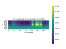
plt.title(f'Mu_d vertical cross section at y={y_slice}')
plt.imshow(Mu_d[:,y_slice,:])
plt.yticks(np.arange(np.shape(Mu_d)[0])[::10],np.round(np.array(getvar(wrf_file,'ZNU'))[::10],2))
plt.ylabel(r'$\eta$')
plt.xlabel('x-coordinate')
plt.colorbar()
I see that there is variation in \mu_d verically about half as much as there is horizontally, and there is almost no variation below critical \eta level (0.2), which would run into contradiction that it is just a horizontally varying 2D variable.
I am trying to close the budgets on momentum and temperature, and have been working under the assumption that \mu_d contains in itself the density and the determinant of the Jacobian transformation to write the governing equations in flux form, following
Numerically consistent budgets of potential temperature, momentum, and moisture in Cartesian coordinates: application to the WRF model.
\mu_d = -g \rho_d |J| ; |J|=dz/deta This is the same as the equation for gradient of geopotential, but the \mu_d I get this way varies in all 3 dimensions.