Hi everyone,
I am new to working with WRF and am currently trying to replicate the results of a paper that shows the output of a passive tracer at a flow rate of 10,000 kg/hr. The paper can be found here: (paper link).
To replicate the study, I first ran a simulation under conditions that are similar to those described in the paper. My setup involves an ideal LES case with a domain size of 1.5 x 1.5 km and a resolution of 15 m. I have four tracer plumes emanating from a 2 x 2 (30 x 30 m) point. In comparison, the paper uses a domain size of 2 x 2 km with a resolution of 20 m and four tracer plumes emanating from a 2 x 2 (40 x 40 m) point. From what I can tell, all other settings are consistent with the paper.
The paper does not provide specific code for plotting the plume, so I created my own. Based on previous posts, I interpreted the dimensionless plume output as parts per billion (ppb) of methane in air. Then, to calculate the flow rate and scale the plume to match the paper’s flow rate of 10,000 kg/hr, I used the following code:
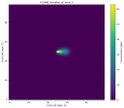
And here is my output at hour 3 with a constant wind speed of 1.5m/s in the x direction:

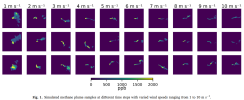
And here is the paper's output at hour 2 or 3 at different wind speeds:

The issue I am facing is that my concentration values are approximately 33 times smaller than those reported in the paper. While I understand my simulation parameters differ slightly from the paper's, I expected my results to be more similar.
Can anyone help me identify whether my assumptions or logic might be incorrect when calculating the flow rate and concentration of the tracer plume? Any feedback or guidance would be greatly appreciated!
I am new to working with WRF and am currently trying to replicate the results of a paper that shows the output of a passive tracer at a flow rate of 10,000 kg/hr. The paper can be found here: (paper link).
To replicate the study, I first ran a simulation under conditions that are similar to those described in the paper. My setup involves an ideal LES case with a domain size of 1.5 x 1.5 km and a resolution of 15 m. I have four tracer plumes emanating from a 2 x 2 (30 x 30 m) point. In comparison, the paper uses a domain size of 2 x 2 km with a resolution of 20 m and four tracer plumes emanating from a 2 x 2 (40 x 40 m) point. From what I can tell, all other settings are consistent with the paper.
The paper does not provide specific code for plotting the plume, so I created my own. Based on previous posts, I interpreted the dimensionless plume output as parts per billion (ppb) of methane in air. Then, to calculate the flow rate and scale the plume to match the paper’s flow rate of 10,000 kg/hr, I used the following code:
Python:
def ppb_to_kgperm2(ppb):
    """
    Convert methane concentration from parts per billion (ppb) to kilograms per square meter (kg/m^2).
    Parameters:
    ppb (float): Methane concentration in parts per billion (ppb).
    Returns:
    float: Methane concentration in kilograms per square meter (kg/m^2).
    """

    M_TO_CM = 1E2  # Conversion factor from meters to centimeters (1 meter = 100 cm).
    CH4_MOLMASS = 16.04  # Molecular mass of methane in grams per mole (g/mol).
    UNIT_TO_PPB = 1E9  # Conversion factor for parts per billion (1 ppb = 1E-9 of the total).
    AVOGNUM = 6.022e23  # Avogadro's number: number of molecules in one mole (molecules/mol).
    AIR_MOLECULES = 2.1E25  # Average number of air molecules per square centimeter in the atmosphere.
    # Calculate the methane concentration in kg/m^2:
    # 1. Convert ppb to the number of methane molecules per cm^2 using AIR_MOLECULES.
    # 2. Use Avogadro's number to convert molecules to moles.
    # 3. Multiply by the molecular mass of methane to get mass in grams.
    # 4. Convert mass from grams to kilograms.
    # 5. Adjust units from cm^2 to m^2 by squaring the conversion factor from meters to centimeters.
    kg_m2 = ppb * M_TO_CM**2 * AIR_MOLECULES / AVOGNUM / UNIT_TO_PPB * CH4_MOLMASS / 1000
    return kg_m2

# Since domain is 1.5 x 1.5 km
x = 1500
y = 1500
# Scale factor to get the flow rate to be 10k kg/hr
scaleFactor = 0.886109764
if __name__ == "__main__":

    # Open the WRF output file
    ncfile = Dataset(_input)

    # Extract the times variable from the WRF output file
    times = getvar(ncfile, "times", ALL_TIMES)

    for hour, time in enumerate(times):

        # Extract the 3D PLUME variable in units of parts per billion (ppb)
        plume = getvar(ncfile, "PLUME", timeidx=hour) * scaleFactor
        # Extract the height variable (z) for the current time index
        z = getvar(ncfile, 'z', timeidx=hour)
        # Calculate the vertical thickness of each layer (dz) by taking the difference along the vertical axis
        # Prepend a zero to ensure the array has the correct shape
        dz = np.diff(z.data, axis=0, prepend=0)
        # Perform vertical integration of the plume data to obtain a 2D representation
        # The integration multiplies the plume concentration by the layer thickness (dz)
        plume_2d = (plume.data * dz).sum(axis=0)
        # Convert the integrated 2D plume from ppb to kilograms per square meter and calculate the total tracer mass
        # The total mass is computed as the sum over the scaled plume values, scaled by the dimension area (x * y)
        # Multiply by dz to account for the thickness of each vertical layer
        total_tracer_mass = np.sum(ppb_to_kgperm2(plume_2d)) * x * y
        print(f"Q: {total_tracer_mass / hour} kg/hr")

        # Plot the 2D plume data
        plt.figure(figsize=(10, 8))
        plt.imshow(plume_2d, origin='lower', cmap='viridis') # , vmin=0, vmax=2000
        plt.title(f'PLUME Variable at Hour {hour}')
        plt.xlabel('Grid Cell Index (X)')
        plt.ylabel('Grid Cell Index (Y)')
        plt.colorbar(label='Concentration (ppb)')
And here is my output at hour 3 with a constant wind speed of 1.5m/s in the x direction:

And here is the paper's output at hour 2 or 3 at different wind speeds:

The issue I am facing is that my concentration values are approximately 33 times smaller than those reported in the paper. While I understand my simulation parameters differ slightly from the paper's, I expected my results to be more similar.
Can anyone help me identify whether my assumptions or logic might be incorrect when calculating the flow rate and concentration of the tracer plume? Any feedback or guidance would be greatly appreciated!
