Artifacts in U and V fields of wrfinput_d01

[Chris Thomas]

I am running real.exe using met_em files generated from data on isobaric vertical levels. These levels are at 1000, 975, 950, 925, 900, 850, ... hPa. The lower levels of the U and V fields contain artifacts. I have attached a screenshot that shows, left to right, the U field (lowest level) in wrfinput_d01, and the UU (lowest level) and PMSL fields in the corresponding met_em file . One can see artifacts in the U field south of Australia and in the tropical cyclone off the north-east coast. These artifacts seem to be related to the PMSL field (right-hand panel in the screenshot). Similar artifacts exist in the V field of wrfinput_d01. These artifacts become less apparent and then disappear with increasing vertical level. There are no features apparent in any of the other fields in the met_em file that correspond to these artifacts. I have also attached a copy of namelist.input. Any ideas?
Chris

 

[kwerner]

Hi,
Can you let me know which version of WRF you are using? Thanks!

 

[Chris Thomas]

My apologies for taking so long to reply. I am using 4.1.2.

Without thinking about it too much, I guess it is a bit strange that the first 2 or 3 isobaric levels of these input data are actually below the surface in the low pressure system. But should real.exe handle this?

This is not a huge problem for me now because I changed to using non-isobaric model-level data from the same dataset.

 

[kwerner]

I *think* that the real program should be able to resolve that issue, but I will run it by our real.exe specialist to see if they have any thoughts.
I'm glad you have a way around this for now, though!

 

[davegill]

Chris,
The artifacts that you see are due to the interaction of the horizontal surface pressure features with the vertical interpolation. Take a look at the following presentation, slides 4 and 5:
https://www2.mmm.ucar.edu/wrf/users/tutorial/202001/wang_runtime_options.pdf

The problem is due to the horizontal discontinuity of the vertical indexes of neighboring grid points when using different vertical levels (from the first guess data) for the same k-index for the WRF computational surfaces (usually the first few levels near the surface). This occurs when the WRF topography (and therefore the WRF surface pressure) is changing in a dramatically different way than the first guess topography (the first guess surface pressure).

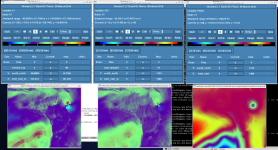
In banded pressure regions (such as the artifact that seems to follow a 2-4 hPa wide zone, I could not see exactly due to the image resolution), those grid cells that are all using the same first guess vertical levels for the interpolation give that resulting red-banded value for the U field.

The first guess isobaric data traditionally does not have well-matched values at the surface and at the nearby constant pressure surface as it intersects the surface. Compounding this is the influence of interpolating to a second surface (from first guess to WRF). The WRF topo can easily be 500 m above or below the first guess. When the WRF model topo is below ground, a simple assumption about a constant U V extrapolation is used. When the WRF model topo is well above the first guess surface, then free atmosphere winds are used (as opposed to something more appropriate to the surface layer). Even without a topo difference (such as over the ocean), the vertical selection of the trapping pressure levels from the first guess will give the artificial elevation shift.

This is what you are seeing. These artifacts are always most obvious over the ocean, as there are no other competing problems. There are interpolation options that are available. The good news is that the model does not need to be run, the real program can be run for a single time period - until you get the desired results. So this experimentation is relatively cheap. As you have found, another solution is to use first guess data that does not have these thick, flat input surfaces (i.e. use native model coordinate data, as opposed to the processed isobaric fields).