Hi everyone,
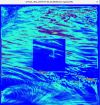
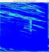
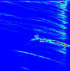
I am running WRF with 3 two-way nested domains and I am experiencing an issue with precipitation fields. When plotting accumulated precipitation over the parent domain (d01), I clearly see square-shaped discontinuities corresponding exactly to the nested domains (d02 and d03). Inside the nested areas, precipitation from the parent domain is almost completely suppressed. The same effect occurs between d02 and d03. It looks like precipitation is being “overwritten” within each child domain area, creating sharp artificial boundaries.
Here is my configuration:
WRF configuration:
Boundary configuration:
My questions:
Thank you very much for your help !
I am running WRF with 3 two-way nested domains and I am experiencing an issue with precipitation fields. When plotting accumulated precipitation over the parent domain (d01), I clearly see square-shaped discontinuities corresponding exactly to the nested domains (d02 and d03). Inside the nested areas, precipitation from the parent domain is almost completely suppressed. The same effect occurs between d02 and d03. It looks like precipitation is being “overwritten” within each child domain area, creating sharp artificial boundaries.
Here is my configuration:
WRF configuration:
- max_dom = 3
- Two-way nesting (feedback = 1)
- smooth_option = 0
- d01: 15 km
- d02: 5 km
- d03: 1.67 km
- parent_grid_ratio = 1, 3, 3
- parent_time_step_ratio = 1, 3, 3
- mp_physics = 8
- cu_physics = 1 (Kain-Fritsch) for d01
- cu_physics = 0 for d02 and d03
Boundary configuration:
- specified = .true., .false., .false.
- nested = .false., .true., .true.
My questions:
- Is this behavior expected with two-way nesting (feedback = 1)?
- Could feedback be suppressing parent-domain precipitation inside child-domain areas?
- Should smooth_option be enabled? Could this be related to differences in convective parameterization between d01 (KF on) and d02/d03 (explicit convection)?
Thank you very much for your help !