Hi WRF support,
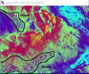
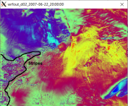
Recently, I noted there are some unphysical stripes (where the velocity of a particular component is some magnitude at one point while it is the magnitude but the opposite direction at the neighboring grid point) in my 3D U and V fields when viewing a wrfout file using NCVIEW (see below. The domain has a 3-km resolution in x and y. The plotted velocity range is from -10 to 10 m/s for both components). At first, I thought these are related to the horizontal staggering of the grids since the clearest stripes in U are mostly north-south orientated and the stripes in V are mostly west-east orientated. These stripy features will average out nicely when I de-stagger the U and V fields along their respective i and j directions.
I did a few tests and found out that the clearest stripes usually occur at where the component speed is small (< 1 m/s). They seem to appear after midday and wane during the evening hours and disappear at higher altitudes. I thought these sort of make sense since the opposite velocities of the same magnitude will average out to be a small number, and convection resulting from daytime heating usually adds frictional drag to boundary-layer winds and wind speed usually increases with height.
I was just wondering if the strange-looking stripes in the staggered U and V fields play a role in the calculation of other fields or it is the de-staggered components that are used in the calculations? I did consider these might be numerical noise and could be removed using diff_6th_opt=2, but I wasn't sure if it is a good idea. I am running a real-case simulation using WRF 4.2.1. The namelist.input I used is attached below.
Any clarification would be greatly appreciated.
Thanks,
David