ecmaggioni
New member
Dear all,
in our modelling configuration we run an ensemble with WPS/WRF 3.9, using different input data, coming from the GFS ensemble, 1 degree of resolution. The area is the Italian region, and during winter we have the problem of the snow cover surfaces. Using the data coming from GFS ensemble at 1 degree, snow cover is too coarse, and it happens that great part of northern Italy is covered by snow, but in reality only small areas in the Alps are covered by snow.
To avoid the problem, we used the possibility offered in WPS to ingest different types of data. We extracted a grib from gfs 0.25 degree with only Water equivalent of snow depth (WEASD), and we run metgrid program using both of the data sources: "FILE", which is from gfs ens, without snow cover, and "SNOWHIRES", which is from gfs 0.25, with only snow cover:
&metgrid
fg_name = 'FILE', 'SNOWHIRES'
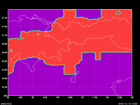
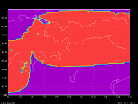
The result with WPS3.9 and WRF3.9 was good, and you can see the difference in the output of WRF model, first wrfout file produced: figure "snowens.png" is the snow cover using only gfs ens (we have a lot of snow cover in the western lowlands, e.g), and "snow_0p25.png" is the snow cover using WEASD coming from gfs 0.25 degree.
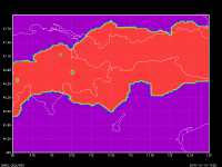
We are using the same strategy with WPS4.0.2, but the results are not what we expected (figure snow_wrf_4p0.png): in general we have more snow covered areas, for example in the area near the Garda Lake or in the area of the Bavaria, and the interpolation is different, with a less smoothing effect than in WPS 3.9. Do you have any suggestion about this different behaviour between WPS3.9 and WPS4.0?
We were thinking about a different treatment of the variables by metgrid, but the part related to snow in METGRID.TBL file is pretty much the same:
name=SNOW
interp_option=four_pt+average_4pt
masked=water
interp_mask=LANDSEA(0)
fill_missing=0.
flag_in_output=FLAG_SNOW
Thanks for the help
Enrico


