You are using an out of date browser. It may not display this or other websites correctly.
You should upgrade or use an alternative browser.
You should upgrade or use an alternative browser.
See the bottom of the WRF-Solar page for a contact regarding WRF-Solar.
But I'm running WRF without WRF-Solar, or is the conversion efficiency about PV panels inside WRF-BEP&BEM itself realized through WRF-Solar?See the bottom of the WRF-Solar page for a contact regarding WRF-Solar.
Here is the PV_FRAC_ROOF in URBPARM.TBL&URBPARM_LCZ.TBLSee the bottom of the WRF-Solar page for a contact regarding WRF-Solar.

The solar panel roof scheme in WRF-BEP/BEM is separated from the WRF-Solar. They are not connected. I think the conversion rate is hard-coded inside the solar panel roof submodule in BEP/BEM code. I am not sure how the value is determined, which is a question for Andrea Zonato. You may want to directly email him.
andreazonato
New member
Hello all,
the variable name is effpv=0.19, hardcoded inside module_sf_bem.F90.
And the energy saving, in W/m^2, is EP_PV_URB3D
Andrea
the variable name is effpv=0.19, hardcoded inside module_sf_bem.F90.
And the energy saving, in W/m^2, is EP_PV_URB3D
Andrea
thank you!I would like to ask how the PV_FRAC_ROOF inside URBPARM.TBL&URBPARM_LCZ.TBL is set? For example, to set a 60% PV roof ratio, how does it pick this 60% area on the roof of a city?Hello all,
the variable name is effpv=0.19, hardcoded inside module_sf_bem.F90.
And the energy saving, in W/m^2, is EP_PV_URB3D
Andrea
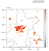
thank you. And I would like to ask if it is normal to have a EP_PV_URB3D (w/m2) of about 20 with 50% rooftop PV installed as shown? And all I have viewed in other people's papers the EP_PV_URB3D is within 5w/m2. I am curious why the result is so big. And the ncl code is below:the current PV_FRAC_ROOF value in the table is set based on the case study from Andrea's recent study. this parameter is tunable based on each city's situation. If you set it to 60%, then it assumes each urban grid will have a uniform 60% of roof area with PV panels.

load "$NCARG_ROOT/lib/ncarg/nclscripts/csm/gsn_code.ncl"
load "$NCARG_ROOT/lib/ncarg/nclscripts/wrf/WRFUserARW.ncl"
begin
;
; The WRF ARW input file.
; This needs to have a ".nc" appended, so just do it.
a = addfile("wrfout_d03_2023-07-28_02:00:00_50solar","r")
b = addfile("wrfout_d03_2023-07-28_02:00:00_original","r")
; We generate plots, but what kind do we prefer?
type = "x11"
; type = "pdf"
; type = "ps"
; type = "ncgm"
; wks@wkWidth = 3600
; wks@wkHeight =3600
; wks = gsn_open_wks(type,"plt_Surface1")
wks = gsn_open_wks(type,"EP_PV_URB3D")
gsn_define_colormap(wks,"BlueWhiteOrangeRed") ; overwrite the .hluresfile color map
; Set some basic resources
res = True
; res@NoHeaderFooter = True ; Switch headers and footers off
res@tmXBLabelFontHeightF = 0.02 ;set the size of x-Axis words
res@tmYLLabelFontHeightF = 0.02 ;set the size of y-Axis words
res@lbLabelsOn = True
res@lbTitleOn = True
res@lbTitleString = "EP_PV_URB3D"
res@lbLabelBarTitlesetF = 0.02 ; 调整标题与labelbar之间的距离
; res@lbLabelFontHeightF = 0.02 ;set the size of label bar words
res@pmLabelBarWidthF = 0.15
res@pmLabelBarHeightF = 0.87
res@lbOrientation = "vertical"
res@pmLabelBarSide = "Right"
res@pmLabelBarOrthogonalPosF = -0.03
; res@pmLabelBarParallelPosF = 0.1
pltres = True
pltres@FramePlot = False
mpres = True
;;;;;;;;;;;;;;;;;;;;;;;;;;;;;;;;;;;;;;;;;;;;;;;;;;;;;;;;;;;;;;;;
; What times and how many time steps are in the data set?
times = wrf_user_getvar(a,"times",-1) ; get all times in the file
ntimes = dimsizes(times) ; number of times in the file
;;;;;;;;;;;;;;;;;;;;;;;;;;;;;;;;;;;;;;;;;;;;;;;;;;;;;;;;;;;;;;;;
do it = 0,ntimes-1,1 ; TIME LOOP
print("Working on time: " + times(it) )
res@TimeLabel = times(it) ; Set Valid time to use on plots
;;;;;;;;;;;;;;;;;;;;;;;;;;;;;;;;;;;;;;;;;;;;;;;;;;;;;;;;;;;;;;;;
; First get the variables we will need
ep_pv_urb3d_a = wrf_user_getvar(a,"EP_PV_URB3D",it) ; T2 in Kelvin
slp = wrf_user_getvar(a,"slp",it) ; slp
ep_pv_urb3d_b = wrf_user_getvar(b,"EP_PV_URB3D",it) ; T2 in Kelvin
ep_pv_urb3d = ep_pv_urb3d_a - ep_pv_urb3d_b
; Plotting options for T
opts = res
opts@cnFillOn = True
; opts@ContourParameters = (/ -1., 1., .1./)
opts@cnLevelSelectionMode = "ManualLevels" ; manually set cn levels
opts@cnMinLevelValF = -20. ; min level
opts@cnMaxLevelValF = 20. ; max level
opts@cnLevelSpacingF = 1 ; contour level spacing
opts@gsnSpreadColorEnd = -3 ; End third from the last color in color map
opts@lbOrientation = "vertical"
opts@pmLabelBarSide = True
contour_ep_pv_urb3d = wrf_contour(a,wks,ep_pv_urb3d,opts)
delete(opts)
; MAKE PLOTS
plot = wrf_map_overlays(a,wks,(/contour_ep_pv_urb3d/),pltres,mpres)
; Set up map resources
plres = True
plres@gsLineColor = "black"
plres@gsLineThicknessF = 1.5
plotshp = gsn_add_shapefile_polylines(wks,plot, shpdir, plres)
draw(plot)
frame(wks)
;;;;;;;;;;;;;;;;;;;;;;;;;;;;;;;;;;;;;;;;;;;;;;;;;;;;;;;;;;;;;;;;
end do ; END OF TIME LOOP
end
Thank you!And I have a new question about EP_PV_URB3D value as above.Hello all,
the variable name is effpv=0.19, hardcoded inside module_sf_bem.F90.
And the energy saving, in W/m^2, is EP_PV_URB3D
Andrea
Sorry for the late reply. The EP_PV_URB3D value depends on the specific location, time, and environmental conditions (e.g., cloud). This is probably a question for @andreazonato . I do not have much experience with a "normal" EP_PV_URB3D value.
Thank you so much! and I also want to know what's the Governing Equations or code of the PVpanel in WRF?Sorry for the late reply. The EP_PV_URB3D value depends on the specific location, time, and environmental conditions (e.g., cloud). This is probably a question for @andreazonato . I do not have much experience with a "normal" EP_PV_URB3D value.
You can take a look at the source code for module_sf_bep_bem.F: WRF/phys/module_sf_bep_bem.F at master · wrf-model/WRF
just search the keyword "EP_PV_URB3D"
just search the keyword "EP_PV_URB3D"
