Change in spec_zone of lateral boundary conditions during runtime

[CWeiss]

Dear all,

I've a question concerning the lateral boundary conditions for a real case run.

I'm running WRF Verion 4.1 on a distributed memory HPC system.

My region of interest is the Great Rift Valley in Ethiopia.

While running wrf.exe, my lateral boundary conditions changed in the spec_zone. If I understood the documentation (https://www2.mmm.ucar.edu/wrf/users/docs/user_guide_V3/users_guide_chap5.htm#Phys -> Lateral Boundary Condition Options d) ), that's usually the region defined and fixed by the input data. I use the HRES analysis from the ECMWF as input data.

After more than 24h runtime, the values for some variables are completely off in the spec_zone. One example is the skin temperature. I'll get values up to 372 K whereas the input data shows values up to 320 K at the same time and area. So the boundary conditions seem to be adapted although they should be fixed.

Does anyone has an idea what happened here?

I'm not in an urgent need but rather interested.
I actually solved it with increasing the layer top from 40hPa to 20hPa (what I should have done in the first place), but still wondering what could be reason for the adaption in the boundary conditions before. I thought of a reflection at the model top or something like this.
Furthermore, it seems that the spec_zone is not fixed after real.exe.

I'll attach my namelist, However, for my "successful" run I changed some more things than just the model top.
I'll also attach a plot generated with ncview that shows in the left hand side (western lateral boundary condition) the abrupt increase of the skin temperature

If more information is needed I'll be happy to provide anything I can.

Looking forward to an answer!
Cheers,
Cornelius

 

[davegill]

This is will a back and forth process.

The lateral boundary conditions do not directly control the physics fields, such as the skin temperature. The lateral boundary conditions in WRF control the dynamics fields that require horizontal differencing to advance the state. It is absolutely possible that one (some / all) of these dynamic fields is (are) having a bad influence on your physics variables.

Look at horizontal (in eta space) plots of the dynamics fields (such as U, V, W, T, PH, QVAPOR, MU). Do the boundaries look discontinuously incorrect? Perhaps you could post a few for us to see. For the 3d fields, look at k=1, k=the top-most-valid-layer, and a middle layer.

 

[CWeiss]

Thanks for your reply and sorry for posting the wrong variable.

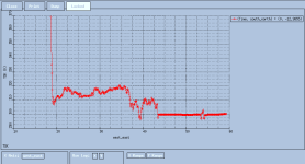
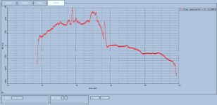
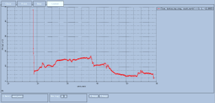
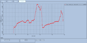
As you recommended I had a look at some dynamic fields. Some of them exhibit a discontinuously behavior as well. However, just in the lower layers close to the surface for the 3D fields (k=1 or 2).
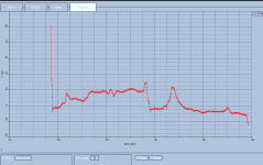
I'll get for example a negative water vapor mixing ration (QVAPOR) or pretty high geopotential perturbations (PH). I'll attach some plots for those and for perturbation of Theta (T), x-wind component (U, which could be realistic) and perturbation of dry air mass in a column (MU).

 

[davegill]

OK, we are getting somewhere! As you indicate, there is a unphysical discontinuity for the T field on th western side of your domain. The PH and MU fields look suspect, but they could just be responding to the T field. We are going to focus on the T field (almost a potential temperature field).

We want to compare a vertical profile from an appropriate grid point of the input data (from metgrid) with a vertical profile from the output of the real program (wrfinput_d01). The real program is responsible for the generation of the lateral boundaries and the initial conditions. What we want to see is where the problem is occurring. Is the data bad in metgrid originally? Does valid data come in from metgrid, and it gets messed up by real?

1. On the western side of your domain (preferably in an area of high pressure), pick a point that is as close to zero elevation as possible. If you have an ocean point, great. If not, as low as you can go is preferred.
Q: Why the western side of the domain?
A: Your discontinuities look really bad on the western side.

2. Get a vertical profile of temperaure from metgrid. My toy domain has an ocean point on the eastern boundary. Instead of my point "(73,10)", you would use "(1,some-j-value-that-is-appropriate)".

ncdump -v TT -f f -b f met_em.d01.2000-01-24_12:00:00.nc | grep "(73,10,"
    296.4829,  // TT(73,10,1,1)
    295.6098,  // TT(73,10,2,1)
    294.3799,  // TT(73,10,3,1)
    292.8598,  // TT(73,10,4,1)
    291.2932,  // TT(73,10,5,1)
    289.7114,  // TT(73,10,6,1)
    288.0058,  // TT(73,10,7,1)
    286.2832,  // TT(73,10,8,1)
    282.7404,  // TT(73,10,9,1)
    278.875,  // TT(73,10,10,1)
    277.48,  // TT(73,10,11,1)
    275.3341,  // TT(73,10,12,1)
    272.1397,  // TT(73,10,13,1)
    267.4374,  // TT(73,10,14,1)
    261.7483,  // TT(73,10,15,1)
    255.4195,  // TT(73,10,16,1)
    248.2741,  // TT(73,10,17,1)
    240.3512,  // TT(73,10,18,1)
    231.5113,  // TT(73,10,19,1)
    221.683,  // TT(73,10,20,1)
    216.7149,  // TT(73,10,21,1)
    212.6502,  // TT(73,10,22,1)
    210.5441,  // TT(73,10,23,1)
    209.2305,  // TT(73,10,24,1)
    207.7082,  // TT(73,10,25,1)
    206.8458,  // TT(73,10,26,1)

3. We want to be able to compute with this data, so we are going to use a few linux commands to strip the information down to just the data we want. Here is what my output would look like:

ncdump -v TT -f f -b f met_em.d01.2000-01-24_12:00:00.nc | grep "(73,10," | cut -d "," -f1 | awk '{print $1}'
296.4829
295.6098
294.3799
292.8598
291.2932
289.7114
288.0058
286.2832
282.7404
278.875
277.48
275.3341
272.1397
267.4374
261.7483
255.4195
248.2741
240.3512
231.5113
221.683
216.7149
212.6502
210.5441
209.2305
207.7082
206.8458

4. Once this works, we want the output of that column of both temperature and pressure from metgrid, each saved to a file:

ncdump -v TT -f f -b f met_em.d01.2000-01-24_12:00:00.nc | grep "(73,10," | cut -d "," -f1 | awk '{print $1}' > TT.txt
ncdump -v PRES -f f -b f met_em.d01.2000-01-24_12:00:00.nc | grep "(73,10," | cut -d "," -f1 | awk '{print $1}' > PRES.txt

5. Now, using the same western-side-of-the-domain grid point, repeat this process of collecting a column of data for three fields from the output from the real program. The metgrid program has temperature, so we added the pressure output to be able to compute the potential temperature. For the wrfinput_d01 file, the output potential temperature is available (just offset by 300 K).

ncdump -v T -f f -b f wrfinput_d01 | grep "(73,10," | cut -d "," -f1 | awk '{print $1}'
-4.753143
-4.557922
-4.288544
-3.8927
-3.412537
-2.958038
-2.422546
-1.736786
-0.9671631
-0.07070923
1.016449
2.023224
4.61618
8.804413
12.51184
15.55624
17.65451
19.3934
21.11127
22.73032
24.45306
26.3429
28.56573
32.21539
41.23279
55.6489
72.1694
90.11481
109.3546
129.6359
151.2271
174.2253

The first value, about -4.75 means a potential temperature of 300 -4.75 = 295.25 K. We want this theta-offset field and the two fields that can be used to reconstruct the pressure: P (perturbation) and PB (reference state). The total pressure at any location is the sum of P and PB.

ncdump -v T -f f -b f wrfinput_d01 | grep "(73,10," | cut -d "," -f1 | awk '{print $1}' > T.txt
ncdump -v PB -f f -b f wrfinput_d01 | grep "(73,10," | cut -d "," -f1 | awk '{print $1}' > PB.txt
ncdump -v P -f f -b f wrfinput_d01 | grep "(73,10," | cut -d "," -f1 | awk '{print $1}' > P.txt

Again, for all of the above examples, I have used the point (73,10). You will choose an appropriate location on the western edge of your domain.

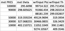
6. Use your favorite plotting package to look at those vertical columns of data. What we want to know is: are the potential temperatures from metgrid (at the specific pressure surface) about the same as the real program (at similar surfaces)? Do not be concerned that the level closest to the ground is off by several hPa, as we asked for data at the half levels. That is probably about 20 m different, and 2-3 hPa lower for the output from real.

7. I picked a few easy vertical locations to check in my data: about 1000, 900, 500, 300, 100 hPa for both metgrid and real. For some of the real locations I gave two surrounding points.

 

[CWeiss]

Hi and sorry for my very late response!!

I compared now the potential temperature from the met_em file and the wrfinput file as you suggested.
I picked a point at the very boudary (i=1) and at a possible low elevation (in my case now 196.2m).
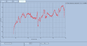
The look pretty similar and I think, the error does not arise from one of the preprocessing steps but rather during runtime of the model itself.
After 30h runtime the suspicious values occur. I checked also the met_em file from this time as is influences the boundary conditions but it looks quite normal.

Any ideas, how the boundary could possibly be changed during runtime? Or what else could be the reason for that whole issue?
Thanks a lot for your help!
Cheers,
Cornelius

 

[CWeiss]

Sorry, an addition to the above listed post:

I meant i = 0, so really at the boundary.
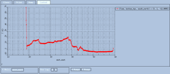
Furthermore, I attach the according plot of the wrfout at this point (i=0, j = 373) after 30h runtime when the weird values at the boundary occur.

 

[davegill]

The fields from the physics schemes are influenced by lateral boundaries, since fields that are forced by the lateral boundaries (loosely: u, v, t, q, height, pressure) are all input the physics schemes. However, a field such as skin temperature does not get nudged directly via a boundary condition.

Is there a problem in the data at a particular time? You have mentioned that the troubles start at 30 h. Let us call this T30.

• If you start the model at T24, do you still see troubles at 6-h into the forecast, at T30?

• If you start the model at T36, does the problem show up?

 

[CWeiss]

Thanks for you reply!
So I tried different start times but ran in similar problems/fields. After some runtime the model crashed.
Independent from the start time. Eg. for T6 as well as for T-6. I have not tried times after T30. However, as far as I remember, the runtime differed until the model crashed. It was not always 30hours. But also not always at the the same "real" time. So for example, once it crashed for 15.1. 12 UTC and once for 14.1. 23UTC.
So neither the runtime nor the "real" time revealed a pattern.
I also checked the input data (EC HRES Analysis with 6h intervall), but that looked fine.

 

[davegill]

For a sanity check, are you able to get access to a different global data set?

Here is a web site at NCAR:
0.25 degree GFS

 

[jessie_zhx]

Hi

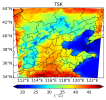
I have recently noticed some interesting behaviors with my WRF-Chem model output. I have set up the model with 2-nested domain and ran a month of simulation in July. The attached plot shows the monthly surface skin temperature (TSK, from WRF-Chem hourly output) averaged during daytime, for the outter domain d1. You can see the edge of the domain, which shows really high values and it seems that it is not nudged well or something is going on. I have found similar patterns for soil moisture and surface temperature as well. When I check the soil moisture in met files and wrfinput_d01 file, they seem normal. It seems that this probably happened during wrf.exe process. I have set up the bdy_control part in the namelist.input as follows:

&bdy_control

spec_bdy_width = 10,

spec_zone = 1,

relax_zone = 9,

specified = .true., .false.,.false.,

nested = .false., .true., .true.,

/

It looks that this might be the reason? I have found this previous post and thought these problems might be similar? Is there any parameter in the bdy_control that I can set to smooth out this gradient in the boundary? Any thoughts or ideas would be appreciated.

Thank you so much,
Jessie

 

[Ming Chen]

Lateral boundary update is only conducted for atmospheric variables. soil and skintemp are predicted by land surface model over the entire model domain including the buffer zone. Unrealistic simulations could be attributed to many factors, including the less accurate forcing from the upper air. usually we skip results in the buffer zone when analyzing the model output.

 

[rdumais63]

Hi

I have recently noticed some interesting behaviors with my WRF-Chem model output. I have set up the model with 2-nested domain and ran a month of simulation in July. The attached plot shows the monthly surface skin temperature (TSK, from WRF-Chem hourly output) averaged during daytime, for the outter domain d1. You can see the edge of the domain, which shows really high values and it seems that it is not nudged well or something is going on. I have found similar patterns for soil moisture and surface temperature as well. When I check the soil moisture in met files and wrfinput_d01 file, they seem normal. It seems that this probably happened during wrf.exe process. I have set up the bdy_control part in the namelist.input as follows:

&bdy_control

spec_bdy_width = 10,

spec_zone = 1,

relax_zone = 9,

specified = .true., .false.,.false.,

nested = .false., .true., .true.,

/

It looks that this might be the reason? I have found this previous post and thought these problems might be similar? Is there any parameter in the bdy_control that I can set to smooth out this gradient in the boundary? Any thoughts or ideas would be appreciated.

Thank you so much,
Jessie

Hi Jessie- did you ever figure out the source of your gradients building up in (what appears to be) the nest's lateral boundary relaxation zone? I am seeing something very similar in my WRF-LES runs. They are much more evident on my LES nest (I am using 4 nests) than on the outer mesoscale nests (usually not noticeable at all on the mesoscale nests) . I have tried different values for spec_bdy_width, spec_zone and relax_zone (up to spec_bdy_width =11). I don't believe it comes from the wrfinput. It could be a product of the vertical nesting I am using (I really think this) , but not absolutely sure. I also am placing model levels < 10 magl, so this could be an issue as well. I am running this configuration at night to avoid convective conditions and model CFL violations (plus a very small timestep). The gradients along some of my edges are not bowing up the model or seemingly causing isues in my interior solution, but they look sloppy, Almost like a box around the edge from demarcating the edge of the relaxation zone. Anyway, they look much as your example for tsk. I also wonder if the 10m and 2m diagnostics work as designed when model levels are placed below 10 magl. Thanks!

 

[jessie_zhx]

Hi Jessie- did you ever figure out the source of your gradients building up in (what appears to be) the nest's lateral boundary relaxation zone? I am seeing something very similar in my WRF-LES runs. They are much more evident on my LES nest (I am using 4 nests) than on the outer mesoscale nests (usually not noticeable at all on the mesoscale nests) . I have tried different values for spec_bdy_width, spec_zone and relax_zone (up to spec_bdy_width =11). I don't believe it comes from the wrfinput. It could be a product of the vertical nesting I am using (I really think this) , but not absolutely sure. I also am placing model levels < 10 magl, so this could be an issue as well. I am running this configuration at night to avoid convective conditions and model CFL violations (plus a very small timestep). The gradients along some of my edges are not bowing up the model or seemingly causing isues in my interior solution, but they look sloppy, Almost like a box around the edge from demarcating the edge of the relaxation zone. Anyway, they look much as your example for tsk. I also wonder if the 10m and 2m diagnostics work as designed when model levels are placed below 10 magl. Thanks!

Hi Sorry for my late reply. My colleague and I did a little bit more investigation. I think the boundary gradient will exist regardless. To minimize the impact, it is better not to do a free run for a longer period of time as this effect will be more significant over time (at least in our case). Also, when processing the data, the few rows of the data at the boundary should probably be discarded. Hope this helps!