em_hill2d_x - behavior with decreasing wind speed

[srinaldi]

Hi all!

I'm playing around with the em_hill2d_x idealized case. In particular, I'd like to reproduce different flow regimes and I started doing this by changing the vertical profile of the wind. I'm having some issues in understanding the output of the simulations when changing the vertical profile of the wind, though.

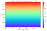
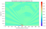
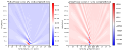
The base case has the wind set as u=10 m/s, and from the vertical profile of the potential temperature I found that N=0.01 s-1, resulting in the lineary parameter u/Nh = 10, where h is the hill height, and giving the well known linear solution.
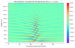
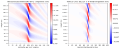
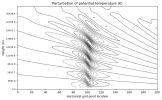
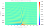
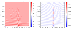
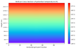
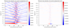
However, if I decrease the wind speed to u=1m/s I get something that I don't well understand, as you can see from the attached figures. First of all, I don't understand why the temperature profile remains the same of the linear case, and then I don't understand what happens at the wind profiles, are there some instabilities arising?

The only thing I changed from the namelist.input is the size of the domain in the west-east direction to have it of 101 gridpoints, then I set the resolution to 1 km and changed the time step accordingly to 6. The hill shape is the same as in the default case, with h=100m and half-width to 5 grid points (so half-width at half-height is 10km if I'm correct).

I hope this question is in line with the topic and the forum.

Thank you very much for your help!

 

[Ming Chen]

I will consult our physics expert and get back to you ....

 

[Pechudin]

I have some experience with mountain meteorology, so I will provide some feedback.

For potential temperature, you should plot perturbation from the base-state potential temperature, instead of raw potential temperature. This is because potential temperature perturbation is proportional to mountain height times d(theta)/dz, which is small compared to the range of theta on the picture (100 K). So just subtract the theta profile you set as the initial condition from the output.

To calculate the theta profile, you can use N=0.01=const. (if it is indeed constant) and integrate the definition of N (you need surface theta as well for the boundary condition).

For the speed plot, how long did you run the simulation and what are the boundary conditions? This velocity field looks good near the ground, but aloft there seem to be reflections (notice the pattern looks like wave field in a 2d channel, when waves can bounce off walls). This can also happen when you have cyclic conditions and wave exits on one side and enters from the other, PACMAN-style. I think open boundary conditions work better? This can also be mitigated by using a larger domain. How large is your domain?