Time shift in wind speed and direction in long-term NDOWN downscaling simulation

[Arty]

Hello WRF Community,

I observed a time shift in wind speed and direction while running a 25-year climate simulation (1991–2016) using NDOWN downscaling from a 21-km parent simulation to a double-nest, 2-way simulation with resolutions of 7 km (d01) and 2.3 km (d02).

During my test runs (3-year runs starting September 2013) with multiple configurations, I did not observe such shifts. In those tests, wind direction and magnitude were coherent with observations. It seems that the shifts appear only over very long simulations.

For my long-term simulation, I used the initial wrfinput* file generated by NDOWN, starting 1991-02. I am now a bit desperate because these are very long and computationally intensive runs. Initially, I regularly checked my outputs for the first decade, and as all seemed normal, I let the runs continue.

I am unsure what could have caused this. Should I have used monthly NDOWN-generated wrfinput files to re-initialize the runs correctly? This seems contradictory to the idea of letting the simulation run after spin-up.

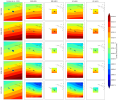
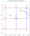
I have attached a couple of figures for d02 (90x90 grid cells, 2.3-km resolution, centered on Tahiti, 17.5°S, 149.5°W) :

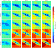
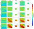
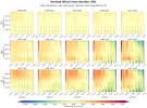
• Average maps of wind speed/vectors over 5 windows of 5 years each.
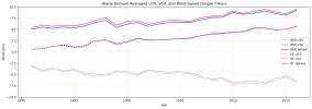
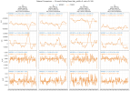
• Yearly domain-average U10MEAN, V10MEAN and SPDUV10MEAN plots showing the observed shift.

Any insight or advice would be warmly appreciated.

Thank you in advance!

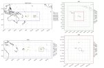
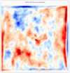
2025/12/06: I added the domains dimensions as a figure for a better understanding.

 

[Arty]

I ran a script to check whether the problem could originate from the original simulation by Dutheil et al., 2019 — as expected, it does not.

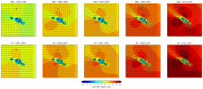
Below, I show a comparison across 5 time windows (rows) for all configurations (BMJ/KF and d01/d02, columns). The shift in wind speed (increase) and direction over the years is clearly visible.

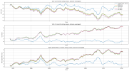
The second figure shows the time series divergence again, while the Dutheil et al., 2019 simulation remains stable over time.

I have also attached my namelist to this post. I am really looking for a way to re-run these long simulations while avoiding this problem.

Thanks again

 

[Hans]

This may seem to be due to the internal variability of RCM, but I am not sure because such a small domain should help suppress drift.

If so, Nudging may be a good approach, but I am not sure if NDOWN can generate the data required for FDDA.

 

[Arty]

This may seem to be due to the internal variability of RCM, but I am not sure because such a small domain should help suppress drift.

If so, Nudging may be a good approach, but I am not sure if NDOWN can generate the data required for FDDA.

As the shift grows in time, I wondered about re-initializing the simulation like every 1-3 years. The domaine is quite small and I did not observe spin-up influence though I did discard the first three months of all my runs.

 

[Arty]

I continued to investigate and am now confident that the problem originates from the initialization file.

I ran several experiments with different topography datasets to evaluate their impact. After these tests, I selected one elevation dataset among the five tested. All five topographies were processed using the same NDOWN downscaling technique; however, I only computed long-term boundary conditions for the default elevation dataset.

I compared the wrfinput* files for the default elevation and the selected “best performance” elevation. I found only minor differences for a few variables, which are summarized below:

2D non-zero variables:
ALBBCK, HGT, MUB, PSFC, SST, TMN, TSK, TSLB, VEGFRA

3D non-zero variables:
P, PB, PH, PHB, P_HYD, T, T_INIT

Spoiler

--- 2D variables ---
ALBBCK:
min=-0.009032249450683594
max=0.0
mean=-2.0071665858267806e-05

HGT:
min=-540.2184448242188
max=400.63916015625
mean=-0.016343258321285248

MUB:
min=-4557.8203125
max=6084.7578125
mean=0.08233832567930222

PSFC:
min=-4569.7109375
max=6097.421875
mean=0.08247341215610504

SST:
min=-1.313568115234375
max=10.784881591796875
mean=-0.3489946722984314

TMN:
min=-2.912261962890625
max=3.923858642578125
mean=-0.36336639523506165

TSK:
min=-1.313568115234375
max=10.784881591796875
mean=-0.3489946722984314

TSLB:
min=-2.912261962890625
max=10.784881591796875
mean=-0.35397687554359436

VEGFRA:
min=0.0
max=13.193550109863281
mean=0.029318999499082565


--- 3D variables ---
P:
min=-11.8223876953125
max=16.8546142578125
mean=4.551762685878202e-05

PB:
min=-4553.265625
max=6078.671875
mean=0.04925476014614105

PH:
min=-78.5
max=104.1875
mean=0.0010619120439514518

PHB:
min=-5299.54345703125
max=3930.270263671875
mean=-0.11829734593629837

P_HYD:
min=-4565.0859375
max=6091.2421875
mean=0.04930104315280914

T:
min=-4.474517822265625
max=3.31463623046875
mean=-5.5714845075272024e-05

T_INIT:
min=-4.474517822265625
max=3.31463623046875
mean=-5.5714845075272024e-05

Importantly, there are no differences at all in the wrfbdy* files between these two configurations.

For further insight, I have attached several figures, including:

• Wind fields (large view)
• Pressure fields (large view)
• One grid pressure time series

These may help illustrate the observed discrepancies.

 

[Ming Chen]

For regional climate simulations using WRF, the 'slab' approach usually gives better results than the 'continuous' approach.

'Slab' means that you run WRF with frequent initialization, for example, you run WRF for the summers during a 20-year period, and each WRF run is initialized at the beginning of each individual year.

'Continuous' run means that you iniialize WRF once, and run the model continuously for 20 years.

It is hard to diagnose the reason for large biases in long-term climate simulations of WRF. Too many factors may get involved.

 

[Arty]

For regional climate simulations using WRF, the 'slab' approach usually gives better results than the 'continuous' approach.

'Slab' means that you run WRF with frequent initialization, for example, you run WRF for the summers during a 20-year period, and each WRF run is initialized at the beginning of each individual year.

'Continuous' run means that you iniialize WRF once, and run the model continuously for 20 years.

It is hard to diagnose the reason for large biases in long-term climate simulations of WRF. Too many factors may get involved.

Thank you, Ming.

This was indeed my fallback solution as well—to re-run the simulations in several shorter segments, perhaps reinitializing every 2–3 years. It is a workable approach, though admittedly a bit cumbersome.

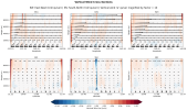
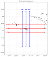
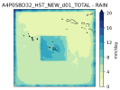
In the meantime, I am still investigating the possible root cause(s) of this drift. Many studies have conducted similar long-term simulations, sometimes over even longer periods (though often at lower resolution), without encountering such issues. In the present case, it seems as though the model is attempting to compensate for spurious forcing at the lateral boundaries. For example, I observe strong updrafts along all boundaries, which—at least to me—suggests that something may have gone wrong quite early in the run. I am also considering whether the LBC generated by NDOWN could be a contributing factor (as shown in the figure below — note that the map encompasses a larger domain than my simulation, but I chose cross-section latitude and longitude ranges that fully cover the model domain).

Lastly, based on your experience, have you encountered similar types of drifts in other work?

 

[Ming Chen]

Hi, Arty,

Thank you for the detailed description of your results.

Some people in NCAR conducted climate simulations using WRF. As far as I know, they either run single-domain simulations using analysis/reanalysis products as the forcing data, or run multi-domain nested simulations with feedback on. In this way, the results between parent-child domain are more consistent.

The lateral boundary issue shown in your result is not uncommon. We did see such kind of resolution-dependent features in many cases, even in the two-way nested cases. To overcome such issues, we usually recommend to set a large child domain, and exclude results along the boundaries when analyzing the simulations.

Hope this is helpful for you.

 

[Arty]

[...] they either run single-domain simulations using analysis/reanalysis products as the forcing data, or run multi-domain nested simulations with feedback on. In this way, the results between parent-child domain are more consistent.

The lateral boundary issue shown in your result is not uncommon. We did see such kind of resolution-dependent features in many cases, even in the two-way nested cases. To overcome such issues, we usually recommend to set a large child domain, and exclude results along the boundaries when analyzing the simulations.

Hope this is helpful for you.

Hi Ming, thank you.

To make sure I’ve fully understood your suggestions, let me restate them:

1. You imply that two-way (feedback) nesting generally produces more consistent results between parent and child domains. That is also what I used. Unfortunately, I still see large discrepancies between d01 and the d02 region within d01 (see attached figure below).
   
   
2. For my specific case, would you however recommend running d02 offline—for example, first run d01 and then use NDOWN for the d02 run—to reduce the latter issue? At the moment, my d01 precipitation field becomes unusable in the d02 area because of this behavior (as shown in the figure).
   
   
3. From the examples you mentioned, I understand that higher resolution can contribute to resolution-dependent features, which might be related to my wind drift problem. Would using a coarser resolution reduce the severity of these boundary issues?
   
   
4. If I understand correctly, you suggest increasing domain size, but I’m not sure whether you mean enlarging d01, d02, or both. At the moment, both of my domains are 120×120, with d02 at three times finer resolution and centered inside d01. I have already cropped out the first 15 border cells as recommended, which leaves me with about 90×90 usable grid points.

Thank you again for your time and help—your explanations are extremely useful.

 

[Arty]

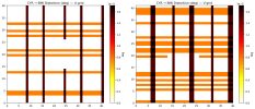
Correction/Clarification: I realize I previously misstated the source of the grid-spacing issue. The figures I shared actually show the distances between common grid points of the 21-km parent domain and the 7-km d01 domain, so there is no “infinite decimal” problem.

However, my question remains: could these slight, local discrepancies between overlapping grid points contribute to the drift observed in long-term simulations? I apologize for the earlier confusion and hope this clarifies the situation.
_________________________________________________________

Sorry, I have one more question. Could the spatial shift I am seeing be related to the fact that the d02 grid spacing is an infinite decimal number (e.g., 7 km / 3 = 2.333… km)? I am wondering whether, over long simulation periods, the slight mismatch between corresponding grid points in d01 and d02 could introduce some numerical noise in the equations or in the computed derivatives.

In my case, I do observe a small bias at some overlapping grid points. The figures below show the magnitude (respectively in meters and degrees) of these biases at common points for the staggered U and V grids between d01 and d02 the 21-km parent domain and the 7-km d01 domain.

It occurred to me that this might play a role, but I’m not experienced enough in numerical methods to assess this properly. It could simply be one of several contributors to the drift, alongside other, more prominent factors.

2025/12/06: Oops, 7 /3 is of course a rational number. As everyone surely noticed, what I meant to highlight was the infinite repeating decimal it produces.
I may need some rest.

 

[Ming Chen]

Hi Arty,
Please see my answers below:

Hi Ming, thank you.

To make sure I’ve fully understood your suggestions, let me restate them:

1. You imply that two-way (feedback) nesting generally produces more consistent results between parent and child domains. That is also what I used. Unfortunately, I still see large discrepancies between d01 and the d02 region within d01 (see attached figure below).

This is a common feature in nesting run. The large discrepancies between d01 and the d02 are attributed to abrupt change in grid interval along the boundary. Currently we have no methods to suppress such kind of discrepancies.

1. 
   
   
2. For my specific case, would you however recommend running d02 offline—for example, first run d01 and then use NDOWN for the d02 run—to reduce the latter issue? At the moment, my d01 precipitation field becomes unusable in the d02 area because of this behavior (as shown in the figure).

I don't think ndown is a good option. This is because it doesn't really address the issues caused by changes in grid interval. It also adds extra efforts to process data and run the model. If a high-resolution run is necessary, then running a nested case with feedback on is a better option.

1. 
   
   
2. From the examples you mentioned, I understand that higher resolution can contribute to resolution-dependent features, which might be related to my wind drift problem. Would using a coarser resolution reduce the severity of these boundary issues?

A coarser resolution that is close to the resolution of the large-scale forcing data can mitigate the boundary issue, although it cannot fully suppress the discrepancy.

1. If I understand correctly, you suggest increasing domain size, but I’m not sure whether you mean enlarging d01, d02, or both. At the moment, both of my domains are 120×120, with d02 at three times finer resolution and centered inside d01. I have already cropped out the first 15 border cells as recommended, which leaves me with about 90×90 usable grid points.

I mean to increase domain size for the child domain. This is because, with a larger domain size, the impact of lateral forcing could be less severe over the interior area of the model domain, and WRF physics and dynamics can fully evolve and dominate the simulation. With a larger child domain, you also have more space to exclude results near the boundary buffer zone.

Thank you again for your time and help—your explanations are extremely useful.

View attachment 19685

 

[Ming Chen]

Hi Arty,

This is another issue I would like to address. You run WRF with the resolution of 21-7-2.333km. Is there any special reason you want to run with the resolution of 2.33km? If not, can you run with the finest resolution of 3km? If so, then you probably can run over a a double-nested domain with the resolution of 9-3km. GFS or ERA5 0.25 degree data can be used to provide large-scale forcing for this resolution.
Some of my colleagues in NCAR actually run WRF for climate simulations with the resolution of 4km, and their results are pretty good. You may contact chliu@ucar.edu (Dr. Changhai Liu) for more information (Hope he can get back to you).
Hope it is helpful for you. I understand that climate simulation is challenging, and good luck in your work!

========================
Sorry, I have one more question. Could the spatial shift I am seeing be related to the fact that the d02 grid spacing is an irrational number (e.g., 7 km / 3 = 2.333… km)? I am wondering whether, over long simulation periods, the slight mismatch between corresponding grid points in d01 and d02 could introduce some numerical noise in the equations or in the computed derivatives.

In my case, I do observe a small bias at some overlapping grid points. The figures below show the magnitude (respectively in meters and degrees) of these biases at common points for the staggered U and V grids between d01 and d02.

It occurred to me that this might play a role, but I’m not experienced enough in numerical methods to assess this properly. It could simply be one of several contributors to the drift, alongside other, more prominent factors.

View attachment 19686

View attachment 19687

 

[Arty]

Hi Arty,

This is another issue I would like to address. You run WRF with the resolution of 21-7-2.333km. Is there any special reason you want to run with the resolution of 2.33km? If not, can you run with the finest resolution of 3km? If so, then you probably can run over a a double-nested domain with the resolution of 9-3km. GFS or ERA5 0.25 degree data can be used to provide large-scale forcing for this resolution.
Some of my colleagues in NCAR actually run WRF for climate simulations with the resolution of 4km, and their results are pretty good. You may contact chliu@ucar.edu (Dr. Changhai Liu) for more information (Hope he can get back to you).
Hope it is helpful for you. I understand that climate simulation is challenging, and good luck in your work!

Hi Ming,

Thanks for your message and for your encouragement.

Unfortunately, I am constrained by the input data I must use: the 21-km South Pacific SST-debiased simulations from Dutheil et al. (2019). These simulations were specifically designed for regional downscaling experiments (historical and RCP8.5) using the pseudo-global-warming method, and they correct the well-known SST bias in GCMs that affects SPCZ location and rainfall intensity. This point is particularly important for my work because my domain is centered on Tahiti, where SPCZ behavior strongly influences local climate.
It also seems worth noting that Dutheil et al. (2021) successfully performed a second (offline) downscaling at 4.2-km resolution over New Caledonia using the same simulation over a 36-year period.

My initial goal was to reach a resolution close to 2.5 km to allow comparison with Météo-France’s AROME model. However, because NDOWN only supports odd refinement ratios, I used a 21→7→2.33… km configuration to approximate this.

That said, I could reconsider the nesting strategy. For instance, I could:

• Use a single 5:1 refinement from 21 km to 4.2 km, or
• Use a double nest with ratios 5 and 3 (or vice versa), reaching 21→4.2→1.4 km (or 21→7→1.4 km), while avoiding rounding issues.

Thank you as well for sharing Dr. Changhai Liu’s contact — I will reach out to him regarding these questions.

In the meantime, I welcome any other questions or insights you may have.

 

[Arty]

Correction/Clarification: I realize I previously misstated the source of the grid-spacing issue. The figures I shared actually show the distances between common grid points of the 21-km parent domain and the 7-km d01 domain, so there is no “infinite decimal” problem.

However, my question remains: could these slight, local discrepancies between overlapping grid points contribute to the drift observed in long-term simulations? I apologize for the earlier confusion and hope this clarifies the situation.

 

[Arty]

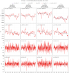
I've continued to work on the issue, but despite several tests, I have not yet been able to identify the root cause. Although I checked the WRFBDY files and found nothing suspicious in the wind components (first figure, red line plots), I clearly observed a shift in time between the original simulation at the boundaries and the d01 boundaries themselves (other figures). I really can't figure it out.



For example, here below are cross-sections of V,W wind on the west boundaries of d01 (quiver for W is magnified 10-fold):





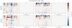
And these below are the anomalies of V wind at boundaries 5 years after simulation start (i.e. 1996/02/01 00:00:00) compared to original data:

 

[Arty]

I went back to the WRF User’s Guide and stumbled upon the following statement in the NDOWN chapter:

“Do not change physics options until after running ndown program.

[...]

The WRF model’s physics options may be modified between runs (the WRF model before ndown and the WRF model after ndown, but do use the same physics from the first run when running ndown), except generally for the land surface scheme option which has different numbers of soil depths depending on the scheme.”

Why must NDOWN be run using the same physics options as the parent domain?

In my case, I changed several physics options in the namelist used for NDOWN, selecting schemes that are better suited to my application. I also noticed that some surface and land-surface schemes differ in their internal structure (e.g., number of layers), and I initially encountered inconsistencies in the wrfinput file produced by NDOWN.

Could these inconsistencies be the origin of the wind drift issue I am observing in my downscaled simulation?

Below I provide the physics options used in the original parent WRF run, followed by the physics namelist actually used for WPS/REAL (wrfndi_d02), NDOWN, and the subsequent WRF runs.

Comparison of physics options​

Physics category	Parent WRF run	REAL / NDOWN / WRF run	Difference
Microphysics (mp_physics)	2 (Purdue–Lin)	6 (WSM6)	Changed
Longwave radiation (ra_lw_physics)	3 (CAM)	4 (RRTMG)	Changed
Shortwave radiation (ra_sw_physics)	3 (CAM)	4 (RRTMG)	Changed
Radiation timestep (radt)	100	5	Changed
Surface layer (sf_sfclay_physics)	1 (MM5 similarity)	1 (MM5 similarity)	Same
Land surface model (sf_surface_physics)	2 (Noah)	1 (Thermal diffusion)	Changed
PBL scheme (bl_pbl_physics)	9 (UW)	1 (YSU)	Changed
Cumulus scheme (cu_physics)	7 (ZM)	2 (BMJ) / 0	Changed
Shallow convection (shcu_physics)	2	0	Changed
Soil layers (num_soil_layers)	4	4	Same
Urban physics	0	0	Same
SST update	1	1	Same
Surface flux option (isftcflx)	1	0	Changed

​

 

[Arty]

I compared the NDOWN outputs for several wind variables and found that, regardless of the namelist physics options used, the results are strictly identical.

This makes me question why not modifying the namelist prior to running NDOWN is recommended, and whether such changes are actually expected to affect the wrfbdy and wrfinput files produced by NDOWN.

 

[Arty]

I also compared the wrfinput files produced by ndown.exe using two different namelists. The files are identical for all atmospheric variables. The only differences occur in soil-related variables, which is expected because the two configurations use a different number of soil layers. The output of the comparison script is shown below.

Spoiler: Comparison of each variables

Opened files successfully


Comparing variables...

Variable ALBBCK: IDENTICAL
Variable CANWAT: IDENTICAL
Variable CF1: IDENTICAL
Variable CF2: IDENTICAL
Variable CF3: IDENTICAL
Variable CFN: IDENTICAL
Variable CFN1: IDENTICAL
Variable CLAT: IDENTICAL
Variable COSALPHA: IDENTICAL
Variable CPLMASK: IDENTICAL
Variable DN: IDENTICAL
Variable DNW: IDENTICAL
Variable DTBC: IDENTICAL
Variable DTS: IDENTICAL
Variable DTSEPS: IDENTICAL
Variable DZS: DIFFERENT SHAPE
BMJ shape: (1, 5)
CYR shape: (1, 4)

Variable E: IDENTICAL
Variable F: IDENTICAL
Variable FCX: IDENTICAL
Variable FNDALBSI: IDENTICAL
Variable FNDICEDEPTH: IDENTICAL
Variable FNDSNOWH: IDENTICAL
Variable FNDSNOWSI: IDENTICAL
Variable FNDSOILW: IDENTICAL
Variable FNM: IDENTICAL
Variable FNP: IDENTICAL
Variable FRC_URB2D: IDENTICAL
Variable GCX: IDENTICAL
Variable HGT: IDENTICAL
Variable ISLTYP: IDENTICAL
Variable IVGTYP: IDENTICAL
Variable LAI: IDENTICAL
Variable LAKEFLAG: IDENTICAL
Variable LAKEMASK: IDENTICAL
Variable LAKE_DEPTH: IDENTICAL
Variable LAKE_DEPTH_FLAG: IDENTICAL
Variable LANDMASK: IDENTICAL
Variable LANDUSEF: IDENTICAL
Variable LU_INDEX: IDENTICAL
Variable MAPFAC_M: IDENTICAL
Variable MAPFAC_MX: IDENTICAL
Variable MAPFAC_MY: IDENTICAL
Variable MAPFAC_U: IDENTICAL
Variable MAPFAC_UX: IDENTICAL
Variable MAPFAC_UY: IDENTICAL
Variable MAPFAC_V: IDENTICAL
Variable MAPFAC_VX: IDENTICAL
Variable MAPFAC_VY: IDENTICAL
Variable MF_VX_INV: IDENTICAL
Variable MU: IDENTICAL
Variable MUB: IDENTICAL
Variable P: IDENTICAL
Variable P00: IDENTICAL
Variable PB: IDENTICAL
Variable PH: IDENTICAL
Variable PHB: IDENTICAL
Variable PSFC: IDENTICAL
Variable P_HYD: IDENTICAL
Variable P_STRAT: IDENTICAL
Variable P_TOP: IDENTICAL
Variable Q2: IDENTICAL
Variable QCLOUD: IDENTICAL
Variable QGRAUP: IDENTICAL
Variable QICE: IDENTICAL
Variable QRAIN: IDENTICAL
Variable QSNOW: IDENTICAL
Variable QVAPOR: IDENTICAL
Variable QV_BASE: IDENTICAL
Variable RDN: IDENTICAL
Variable RDNW: IDENTICAL
Variable RDX: IDENTICAL
Variable RDY: IDENTICAL
Variable RESM: IDENTICAL
Variable SAVE_TOPO_FROM_REAL: IDENTICAL
Variable SEAICE: IDENTICAL
Variable SH2O: DIFFERENT SHAPE
BMJ shape: (1, 5, 120, 120)
CYR shape: (1, 4, 120, 120)

Variable SHDMAX: IDENTICAL
Variable SHDMIN: IDENTICAL
Variable SINALPHA: IDENTICAL
Variable SMCREL: DIFFERENT SHAPE
BMJ shape: (1, 5, 120, 120)
CYR shape: (1, 4, 120, 120)

Variable SMOIS: DIFFERENT SHAPE
BMJ shape: (1, 5, 120, 120)
CYR shape: (1, 4, 120, 120)

Variable SNOALB: IDENTICAL
Variable SNOW: IDENTICAL
Variable SNOWC: IDENTICAL
Variable SNOWH: IDENTICAL
Variable SOILCBOT: IDENTICAL
Variable SOILCTOP: IDENTICAL
Variable SR: IDENTICAL
Variable SST: IDENTICAL
Variable STEP_NUMBER: IDENTICAL
Variable T: IDENTICAL
Variable T00: IDENTICAL
Variable T2: IDENTICAL
Variable TH2: IDENTICAL
Variable TISO: IDENTICAL
Variable TLP: IDENTICAL
Variable TLP_STRAT: IDENTICAL
Variable TMN: DIFFERENT
Dims : ('Time', 'south_north', 'west_east')
dtype : float32
# diffs : 32
Examples (index -> BMJ | CYR):
(0, 56, 62) -> 297.6732482910156 | 285.8190612792969
(0, 56, 63) -> 298.37017822265625 | 286.3839416503906
(0, 57, 62) -> 297.3658142089844 | 285.4075622558594
(0, 57, 63) -> 298.4068298339844 | 286.3055419921875
(0, 58, 57) -> 296.31024169921875 | 284.8380432128906
(0, 58, 58) -> 295.97930908203125 | 284.475341796875
(0, 58, 59) -> 296.8528137207031 | 285.2626037597656
(0, 58, 60) -> 297.9208068847656 | 286.1729431152344
(0, 58, 61) -> 298.8175048828125 | 286.9119873046875
(0, 59, 57) -> 294.763671875 | 283.2769470214844

Variable TOPOSLPX: IDENTICAL
Variable TOPOSLPY: IDENTICAL
Variable TSK: IDENTICAL
Variable TSLB: DIFFERENT SHAPE
BMJ shape: (1, 5, 120, 120)
CYR shape: (1, 4, 120, 120)

Variable T_BASE: IDENTICAL
Variable T_INIT: IDENTICAL
Variable Times: IDENTICAL
Variable U: IDENTICAL
Variable U10: IDENTICAL
Variable UOCE: IDENTICAL
Variable U_BASE: IDENTICAL
Variable U_FRAME: IDENTICAL
Variable V: IDENTICAL
Variable V10: IDENTICAL
Variable VAR: IDENTICAL
Variable VAR_SSO: IDENTICAL
Variable VEGFRA: IDENTICAL
Variable VOCE: IDENTICAL
Variable V_BASE: IDENTICAL
Variable V_FRAME: IDENTICAL
Variable W: IDENTICAL
Variable XLAND: IDENTICAL
Variable ZETATOP: IDENTICAL
Variable ZNU: IDENTICAL
Variable ZNW: IDENTICAL
Variable ZS: DIFFERENT SHAPE
BMJ shape: (1, 5)
CYR shape: (1, 4)

Variable Z_BASE: IDENTICAL

Comparison complete.

 

[Arty]

After nearly three weeks and dozens of test runs, I can confidently rule out the following potential causes.

What is not causing the issue​

• Nesting: removing the d02 nest yields similar wind drift in d01.
• Lateral boundary conditions (LBCs): wrfbdy files produced by NDOWN remain consistent with the original wrfout data.
• Initial conditions (ICs): see details below, particularly regarding SST*.
• CPU allocation: reducing the allocation from 144 to 64 CPUs produces identical results over simulations spanning several months.
• Domain size: similar boundary perturbation patterns appear, and wind drift seems to grow even faster in a 180×180 domain.
• Forcing dataset: a CFSRv2-forced simulation over an equivalent d01 (120×120, 7-km resolution, Tahiti-centered domain) exhibits the same boundary perturbation patterns**.
• Boundary width: increasing bdy_width from 5 to 8 while keeping spec_exp = 0.33 in a CFSRv2-forced simulation still leads to boundary perturbations***.

As is probably clear, I have spent considerable time trying to identify both the origin of the issue and any possible mitigation strategies—without success so far.

In the meantime, following a suggestion from @Ming Chen, I re-launched yearly re-initialized simulations (13-month runs, including a 1-month spin-up). This approach does work. While I am relieved to have a practical workaround that allows me to complete my PhD with coherent downscaled simulations, I remain somewhat disappointed. Something in the model behavior clearly limits results robustness, and it is frustrating not to be able to perform the originally planned fully continuous 25-year run. That said, I recognize that this is part of pushing the boundaries of understanding—and that numerical models are inherently complex systems we must work with as best we can.

Additional technical notes​

* While NDOWN interpolates atmospheric fields for wrfinput and wrfbdy, it does not interpolate SST. Although SST is provided via wrflowinp, WRF initialization actually uses the SST contained in wrfinput. This is an important detail to keep in mind; however, I can assess that an incorrect initial SST—corrected at the next forcing time step—has no significant impact on the simulation output.

** Strong wind-speed fluctuations (resembling “bubbles” of higher and lower wind speeds) are visible in the boundary regions, as shown in the first figure of this post.

*** Increasing bdy_width effectively reduces the decay rate of boundary influence. With spec_exp = 0.33, the boundary impact extends to roughly ~3Δx. I observed pronounced wind anomalies between simulations using bdy_width = 5 and bdy_width = 8, illustrated in the screenshots below for U10 and V10 over a two-month integration.

Broader perspective​

Offline downscaling with NDOWN is a powerful and important capability of the WRF modeling system. In my view, it deserves greater attention, as it enables a wide range of study cases—some of which naturally push the limits of the system. My own setup is admittedly somewhat unusual: I only have access to pre-existing 21-km-resolution wrfout files, from which I generated a two-way double nest, increasing resolution by a factor of 3×3.

Once I complete my PhD (hopefully by mid-2026), I would like to contribute back by sharing feedback based on the difficulties I encountered, with the goal of helping other users through more detailed, experience-based guidance on the use of NDOWN. In particular, I believe the NDOWN chapter of the User’s Guide could benefit from user feedback and a broader description of both its capabilities and limitations. I would be glad to contribute toward improving the overall user experience.

Acknowledgments​

Finally, I would like to express my sincere thanks to NCAR as a whole, and to all the teams whose work underpins the tools, models, and datasets many of us rely on daily. Given the current situation in the US, I want to offer my full support and appreciation. Your work is outstanding and deserves far more recognition than it currently receives. I sincerely hope that the decades of effort invested in these models, infrastructures, and scientific collaborations will continue well into the future.

On a merrier note, I wish everyone a peaceful holiday season and all the best for the upcoming Christmas and New Year.